Cuddling up to Microsoft Excel

Microsoft Excel is like my fussy white cat. She’s hard not to love, but if she’s not worshiped properly she may turn against you. Go too fast, expect a hard swipe and bite.

Don't mess with me... but I *am* purr-bel-icious!

Don’t mess with me… but I *am* purr-bel-icious!


She must not be manhandled; one approaches her with appropriate reverence and respect. First, proffer the finger for sniffing; then hold finger still as she rubs her cheek against it. Only after these formalities am I allowed to get cuddly and lovie with kitty.

I love Excel for the power it has to create quick displays, and return nice results for standard deviation, mean, standard error, etc… but its convoluted ways of labeling can be so annoying! You must approach the graphs with special attention and genuflections.

Want to create a line graph? Then … certainly don’t press line graph; go to XY scatter plot and pick the icon with the curvy lines connecting the dots!

Want to create a bar graph? Then… certainly don’t press bar graph; go to column graph instead. Arrrggghhh.

If you have any tips for using Excel to create good data displays for investigations, please feel free to share them in comments below.

Onward to science fair!

Standard Deviation and Standard Error

Students looking for more advanced analysis on their science fair projects will want to understand standard deviation and standard error.

It’s fine to define measures of central tendency using mean, median, and mode, but what about the spread, or variance, of the data? A box and whisker plot very nicely shows the spread of data in the width of the box (since the box contains exactly half the data), but using standard deviation we can see much more.

Here’s a quick video going over the derivation of standard deviation:

I like to give the students some sense of where these equations come from!

Next, we have standard error. It’s helpful to run through scenario with the students where you imagine “What if we had a very, very large N? How would that affect the Error?” (denominator increasing causes the ratio to decrease – which makes sense, that a large sample size would decrease error). “What if we had a very small standard deviation? The dependent variable returned almost precisely the same value for each trial?” (numerator decreasing also causes the ratio to decrease – again, less error if there’s more consistent correlation between the independent and dependent variables.)

The next video explains how to place error bars on Excel. I don’t know why, but whenever I try to use Excel to place standard error bars according to its default settings, it doesn’t seem to be accurate. You’d think it would be, since there is the option “Error bars – use standard error” – but this option creates the same error for each of the different bars in a bar graph. In most of our science experiments, each bar is going to need its own error measurement because it represents its own set of data…

Someone else on Youtube very nicely explained how to create each bar with its own standard error bar (I’d give him credit here, but I don’t remember the video exactly!), so I used his method to create this explanation here:

Hopefully, advanced 8th grade students who want to be competitive at science fair can apply these ideas to their own data sets.

Hypothesis as Function, displayed as Trendline Equation

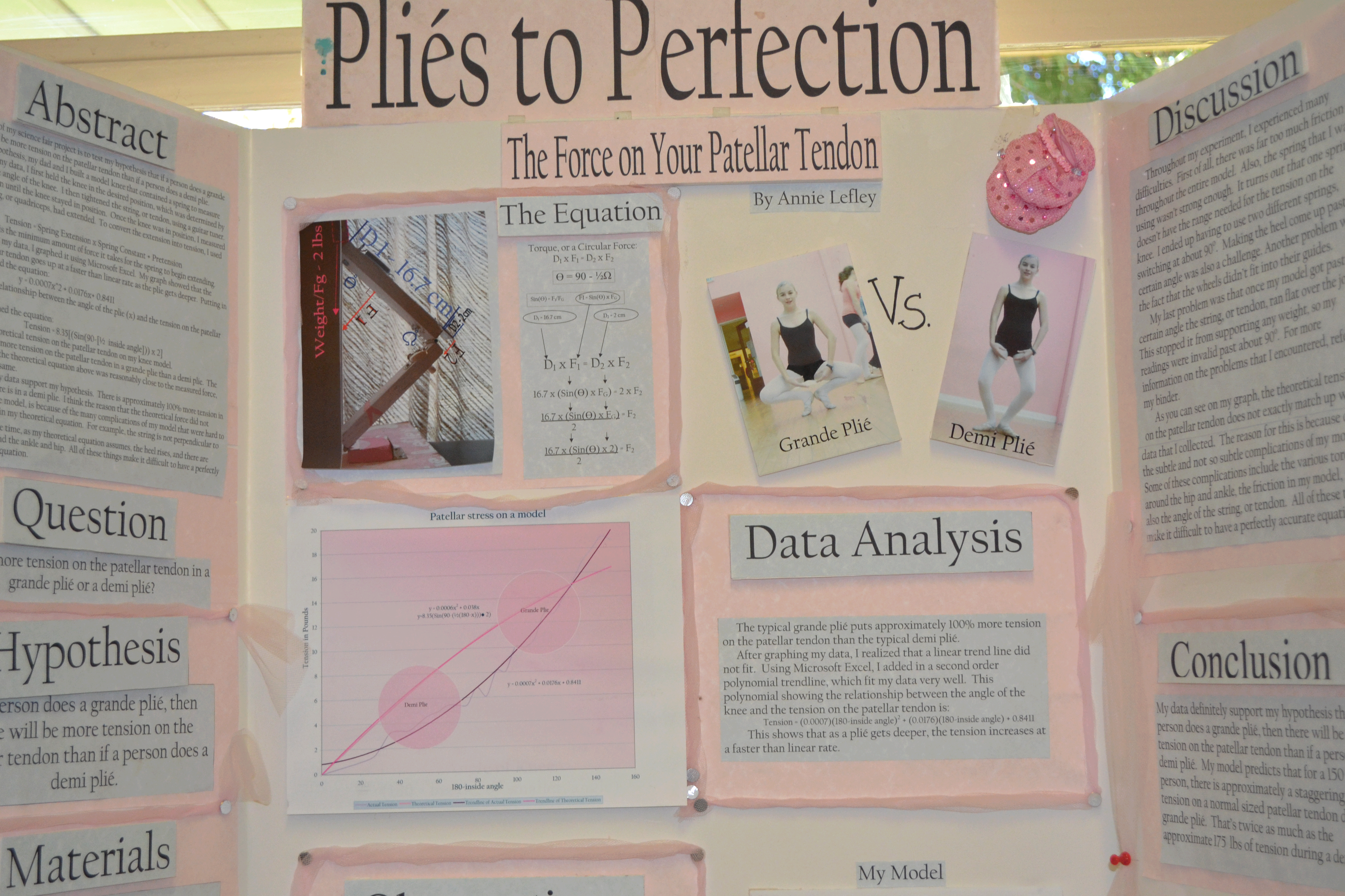
Annie's award-winning project is on www.sciencebuddies.org

Annie’s award-winning project is on www.sciencebuddies.org

I’ve made a video series on Youtube designed to help students analyze their independent investigation results and go beyond a simple bar graph.

Most of my eighth grade students have some notion of the general form of a slope-intercept line equation: y = mx + b.
What they don’t realize, necessarily, is that what they learned in room 309 with Mr. Math Teacher can help them a LOT in their science classroom with me!

To generate a good science fair hypothesis that can be clearly graphed, the independent variable and dependent variable need quantifiable units. That is an entire subject unto itself. Here, I’m going to focus on how I teach students to make a trendline equation once they’ve already identified their independent variable as “what goes on the X axis” and the dependent variable as “what goes on the Y axis”.

The hypothesis is really a proposal that X and Y are correlated in some sort of functional relationship. With the hypothesis, we boldly make a conditional statement “If X, then Y.” If there is a one-to-one correspondence between every X value and a Y value, so that every X returns one and only one Y value, we can say Y is a function of X.

A function can be represented in the form of a table, a graph, or an equation, and in science experiments we commonly progress through exactly those stages: first we collect data in a table, then we graph that data, then (perhaps) we create an equation from that data. Since the equation is a powerful predictive tool, it can be the most important way to summarize the data from an experiment. Of course, caveats apply: the equation may not necessarily hold for extrapolations of variables beyond the experimental set.

Students do feel proud of themselves when they discover the equation that describes the relationship between their independent and dependent variables. They are using the analytic tools of a real scientist and, let’s face it, an equation posted in the Results/Analysis section of a Science Fair display board do always look impressive.

This video playlist shows how to make a trendline equation in Microsoft Excel 2010. Other versions of Excel will be slightly different, but the discussion of finding trendlines can still be relevant:

http://www.youtube.com/watch?v=x9JMf1xD_Gc&list=PL03mSKVZUXBSqBCLe_paf-iymfEbGMokx&index=1

Enjoy!